← EPR Simulation with Igor Pro (the 1999 page) · Site map

EPRSim XOP — what survives

Recovered 6 September 2026 from the two BinHex archives the 1999 page still links to. Version 1.1, April 1996, Oregon Graduate Institute.

The short version. The two archives each hold a compiled plug-in for Classic Mac OS (PowerPC and 68K builds of EPRSim 1.1) and one demo experiment. The plug-ins are binaries only: no C source survived, and neither did the QPOW code they wrapped. The demo experiment is the real find: it is an Igor packed experiment, and inside it are the macro source, two help notebooks written in April 1996 (the full user manual, every one of the 70 QPOW parameters documented), one real experimental spectrum with the QPOW simulation of it, and the isotropic example. Everything below came out of that one 64 KB file, plus the Function Help text stored inside the plug-in.

The data

Wave phm382: 2000 points, 2440–3439.5 G in 0.5 G steps, recorded at 9.105 GHz. The graph in the experiment labelled it “PHM (Type II Cu protein)” — peptidylglycine α-hydroxylating monooxygenase, sample 382. Wave sim1: the QPOW simulation, 500 points at 2.004 G/pt, scaled here to the data's peak.

Back in 1996, this took a minute or so to run on a Mac Quadra. At the end, it played this sound to let you know it was done:

Four seconds of 8-bit mono at 11 kHz, the snd resource that lived inside the plug-in, unchanged. Slot 69 of params turned it on.

Wave IsoWave: the SimulateIso() output for a DMPO-S (thiyl) spin adduct, one nitrogen (a = 14.1 G) and one hydrogen (a = 16.3 G), 30 % Lorentzian. The experiment's graph placed it on a 0–635 G axis; the parameter wave says 0.1 G per point, which is what is drawn here.

Running it again

The params values below (g = 2.036, 2.036, 2.245; A = 40, 40, 525 MHz; natural-abundance copper; 9.105 GHz; 2440–3440 G) fed to the open-source Python package EPRsim on 6 Sep 2026. Every hyperfine line lands where QPOW put it; the widths agree once the linewidth is expressed in EPRsim's convention (8.0 mT Gaussian FWHM here, against QPOW's 130/130/160 MHz plus its strain terms). Correlation with sim1: 0.995. The script is resim_with_EPRsim.py (raw); it took 0.04 s.

No sound is played here. It only took 0.04 seconds to run.

The parameters that produced the simulation

The params wave, 70 slots, exactly as saved. The meanings are your own words from the Function Help. The values that were varied by the macros are slots 8–11 (frequency and g), 18–20 (A) and 47–49 (linewidths): g = 2.036, 2.036, 2.245; A = 40, 40, 525 MHz; linewidths 130, 130, 160 MHz; I = 3/2, two copper isotopes (69 % ⁶³Cu, g-ratio 1.071 for ⁶⁵Cu), quadrupole 5 and −1 MHz, first derivative, Gaussian lines, centre 2940 G, sweep 1000 G.

All 70 slots of params

#	value	meaning (from the 1996 function help)	group
0	1.5	SPINA= Spin of metal nucleus being studied
1	0	SPINB= Spin of superhyperfine nucleus, B
2	0	SPINC= Spin of superhyperfine nucleus, C; C is magnetically different than B
3	0	SPIND= Spin of superhyperfine nucleus, D
4	0	NEB= # of B type atoms
5	0	NEC= # of C type atoms
6	0	NED= # of D type atoms
7	8	CUTOFF= # of linewidths the spectrum is to be calculated over
8	9.105	NU=Frequency at which spectrum was recorded, IN GHZ
9	2.036	GX= g in X direction	PRINCIPLE VALUES OF THE G MATRIX:
10	2.036	GY= g in Y direction	PRINCIPLE VALUES OF THE G MATRIX:
11	2.245	GZ= g in Z direction	PRINCIPLE VALUES OF THE G MATRIX:
12	16	NTR= # of transitions possible considering only nucleus A; if your NTR is too large program will substitute NTR=((SPINA2)+1)*2	PRINCIPLE VALUES OF THE G MATRIX:
13	10	NTH= # of intervals along the Theta direction for which spectra will be calculated. If Theta ranges from 0 to 90 degrees, and NTH is set at 9, there will be 9 intervals, each of 10 deg. Actually, half of this number will be calculated due to interpolation. Four points will be calculated inside each interval as determined by Gaussian quadrature. The maximum value for NTH is 49.	PRINCIPLE VALUES OF THE G MATRIX:
14	1	NPH= # of intervals along the PHI direction when NTH is set at 90 degrees. The number of intervals along the PHI direction is dependent upon THETA as well as NPH: [Sin(THETA)][NPH]; therefore, as THETA approaches zero, the # of intervals decreases. The maximum value of NPH is 15.	PRINCIPLE VALUES OF THE G MATRIX:
15	0	ITH= Initial THETA angle (to calculate only the perpendicular part of the spectrum, ITH should be about 40).	PRINCIPLE VALUES OF THE G MATRIX:
16	1	LTH= Range of THETA integration divided by PI/2; if the Gz coordinate axis is coincident with the Az coordinate axis, the Range = 90 degrees, and LTH =1; if they are noncoincident, the Range = 180 degrees and LTH = 2.	PRINCIPLE VALUES OF THE G MATRIX:
17	1	LPH= Range of PHI integration divided by PI/2; If the Gx and Gy axes are coincident with the Ax and Ay axes, respectively, the Range = 90 degrees and LPH=1, otherwise, the Range = 180 and LPH-2.	PRINCIPLE VALUES OF THE G MATRIX:
18	40	AX= A along X axis	PRINCIPAL VALUES OF HYPERFINE MATRIX FOR THE METAL NUCLEUS (IN MHZ):
19	40	AY= A along Y axis	PRINCIPAL VALUES OF HYPERFINE MATRIX FOR THE METAL NUCLEUS (IN MHZ):
20	525	AZ= A along Z axis	PRINCIPAL VALUES OF HYPERFINE MATRIX FOR THE METAL NUCLEUS (IN MHZ):
21	0	ALPHA	ANGSA= Euler angles which rotate the A matrix from the coordinate system where the G-matrix is diagonal to the coordinate system where the A-matrix is diagonal (if G and A are coincident, these are set equal to zero):
22	0	BETA	ANGSA= Euler angles which rotate the A matrix from the coordinate system where the G-matrix is diagonal to the coordinate system where the A-matrix is diagonal (if G and A are coincident, these are set equal to zero):
23	0	GAMMA	ANGSA= Euler angles which rotate the A matrix from the coordinate system where the G-matrix is diagonal to the coordinate system where the A-matrix is diagonal (if G and A are coincident, these are set equal to zero):
24	0	In X direction	PRINCIPAL HYPERFINE MATRIX VALUES FOR B ATOMS:
25	0	In Y direction	PRINCIPAL HYPERFINE MATRIX VALUES FOR B ATOMS:
26	0	In Z direction	PRINCIPAL HYPERFINE MATRIX VALUES FOR B ATOMS:
27	0	ALPHA	ANGSB=EULER ANGLES FOR B ATOMS:
28	0	BETA	ANGSB=EULER ANGLES FOR B ATOMS:
29	0	GAMMA	ANGSB=EULER ANGLES FOR B ATOMS:
30	0	In X direction	PRINCIPAL HYPERFINE MATRIX VALUES FOR C ATOMS:
31	0	In Y direction	PRINCIPAL HYPERFINE MATRIX VALUES FOR C ATOMS:
32	0	In Z direction	PRINCIPAL HYPERFINE MATRIX VALUES FOR C ATOMS:
33	0	ALPHA	ANGSC=EULER ANGLES FOR C ATOMS:
34	0	BETA	ANGSC=EULER ANGLES FOR C ATOMS:
35	0	GAMMA	ANGSC=EULER ANGLES FOR C ATOMS:
36	0	In X direction	PRINCIPAL HYPERFINE MATRIX VALUES FOR D ATOMS:
37	0	In Y direction	PRINCIPAL HYPERFINE MATRIX VALUES FOR D ATOMS:
38	0	In Z direction	PRINCIPAL HYPERFINE MATRIX VALUES FOR D ATOMS:
39	0	ALPHA	ANGSD=EULER ANGLES FOR D ATOMS
40	0	BETA	ANGSD=EULER ANGLES FOR D ATOMS
41	0	GAMMA	ANGSD=EULER ANGLES FOR D ATOMS
42	5	qdd= 3/2*QZ in MHZ (QZ=quadrapole along the Z axis)	(IN THE COORDINATE SYSTEM WHERE THE QUADRAPOLE TENSOR IS DIAGONAL:)
43	-1	QE=1/2*(QX-QY) in MHZ	(IN THE COORDINATE SYSTEM WHERE THE QUADRAPOLE TENSOR IS DIAGONAL:)
44	0	ALPHA	ANGSQ=Euler angles which rotate the Q tensor from the coordinate system in which the G tensor is diagonal to the coordinate system where the Q tensor is diagonal:
45	0	BETA	ANGSQ=Euler angles which rotate the Q tensor from the coordinate system in which the G tensor is diagonal to the coordinate system where the Q tensor is diagonal:
46	0	GAMMA	ANGSQ=Euler angles which rotate the Q tensor from the coordinate system in which the G tensor is diagonal to the coordinate system where the Q tensor is diagonal:
47	130	IN THE X DIR	LINEWIDTHS ALONG PRINCIPLE DIRECTIONS OF THE G MATRIX (in MHZ):
48	130	IN THE Y DIR	LINEWIDTHS ALONG PRINCIPLE DIRECTIONS OF THE G MATRIX (in MHZ):
49	160	IN THE Z DIR	LINEWIDTHS ALONG PRINCIPLE DIRECTIONS OF THE G MATRIX (in MHZ):
50	1	IDERIV=The derivative of the spectrum (1st or 2nd)	LINEWIDTHS ALONG PRINCIPLE DIRECTIONS OF THE G MATRIX (in MHZ):
51	1.5	GN= Nuclear G-factor for the 1st isotope of the metal.	LINEWIDTHS ALONG PRINCIPLE DIRECTIONS OF THE G MATRIX (in MHZ):
52	1	GR= Ratio of g factors of 2nd isotope to 1st.	LINEWIDTHS ALONG PRINCIPLE DIRECTIONS OF THE G MATRIX (in MHZ):
53	1.071	QR= Ratio of quadrapole moments of the 2nd to 1st.	LINEWIDTHS ALONG PRINCIPLE DIRECTIONS OF THE G MATRIX (in MHZ):
54	0.69	GWT(1)= Fraction of abundance of 1st isotope (if only one isotope, GWT(1) = 1.00).	LINEWIDTHS ALONG PRINCIPLE DIRECTIONS OF THE G MATRIX (in MHZ):
55	2	NIS= Number of isotopes. If NIS=1, only the 1st isotope is calculated, if NIS=2, two isotopes are calculated.	LINEWIDTHS ALONG PRINCIPLE DIRECTIONS OF THE G MATRIX (in MHZ):
56	2940	LCR= Center of spectrum (in Gauss)	LINEWIDTHS ALONG PRINCIPLE DIRECTIONS OF THE G MATRIX (in MHZ):
57	1000	LTOT= Field sweep (width of spectrum) (in Gauss)	LINEWIDTHS ALONG PRINCIPLE DIRECTIONS OF THE G MATRIX (in MHZ):
58	2	HINT= Size of interval for PTS to be plotted (in gauss); program will calculate a point every HINT # of gauss.	LINEWIDTHS ALONG PRINCIPLE DIRECTIONS OF THE G MATRIX (in MHZ):
59	2	In X direction	EPSILN= CONSTANT RELATING THE CORRELATION OF A- AND G-STRAIN:
60	2	In Y direction	EPSILN= CONSTANT RELATING THE CORRELATION OF A- AND G-STRAIN:
61	2	In Z direction	EPSILN= CONSTANT RELATING THE CORRELATION OF A- AND G-STRAIN:
62	0	In X direction	CONSTANT CONTAINING INFORMATION ON THE EXTENT OF A-STRAIN IN MHZ:
63	0	In Y direction	CONSTANT CONTAINING INFORMATION ON THE EXTENT OF A-STRAIN IN MHZ:
64	0.75	In Z direction	CONSTANT CONTAINING INFORMATION ON THE EXTENT OF A-STRAIN IN MHZ:
65	0	In X direction	CTWO=CONSTANT CONTAINING INFORMATION ON THE EXTENT OF G-STRAIN
66	0	In Y direction	CTWO=CONSTANT CONTAINING INFORMATION ON THE EXTENT OF G-STRAIN
67	2	In Z direction	CTWO=CONSTANT CONTAINING INFORMATION ON THE EXTENT OF G-STRAIN
68	0	Gaussian or Lorentzian lineshape. Gaussian = 0, Lorentzian = 1.	CTWO=CONSTANT CONTAINING INFORMATION ON THE EXTENT OF G-STRAIN
69	1	Sound On/Off. If = 1, then Igor will play a bit of the theme from "The Good, the Bad, and the Ugly" when it is done simulating. A value of 0 turns this option off.	CTWO=CONSTANT CONTAINING INFORMATION ON THE EXTENT OF G-STRAIN

The 13 slots of paramsIso

#	value	meaning
0	0.1	X increment (G/pt)
1	1	Phase (1 or −1)
2	2	Number of different nuclei
3	1	Linewidth
4	100	Y max (scale)
5	0	Delta g (shift between nuclei)
6	0.3	Fraction Lorentzian
7	1	Nucleus 1: number of nuclei
8	14.1	Nucleus 1: coupling constant (G)
9	0.5	Nucleus 1: spin
10	1	Nucleus 2: number of nuclei
11	16.3	Nucleus 2: coupling constant (G)
12	1	Nucleus 2: spin

The macro source

The experiment's procedure window: the “Simulation” menu, the three macros, and the two graph windows.

Menu "Simulation"
	"Init Params /1"
	"Simulation /2"
	"Params Wave to Globals /3"
end

Proc InitParams_1(theSimulationWave,theParamsWave)			| makes and initializes global variables assumed by macros below
	String theSimulationWave="sim1", theParamsWave="params"
	Prompt theSimulationWave, "Simulation Wave:"
	Prompt theParamsWave, "Parameters Wave:"
	String/G SimulationWave=theSimulationWave, ParamsWave=theParamsWave
	print SimulationWave, ParamsWave
End

Proc InitParams_2(thefreq, thegx,thegy,thegz,theax,theay,theaz,thelinewidth_x, thelinewidth_y, thelinewidth_z)			| makes and initializes global variables assumed by macros below
	Variable thefreq=9.105, thegx=2.036,thegy=2.036,thegz=2.245,theax=40,theay=40,theaz=525,thelinewidth_x=130, thelinewidth_y=130, thelinewidth_z=160
	Prompt thefreq, "Frequency:"
	Prompt thegx, "gx:"
	Prompt thegy, "gy:"
	Prompt thegz, "gz:"
	Prompt theax, "Ax (in MHz):"
	Prompt theay, "Ay (in MHz):"
	Prompt theaz, "Az (in MHz):"
	Prompt thelinewidth_x, "Linewidth X (in MHz): "
	Prompt thelinewidth_y, "Linewidth Y (in MHz): "
	Prompt thelinewidth_z, "Linewidth Z (in MHz): "
		
	Variable/G freq=thefreq, gx=thegx,gy=thegy,gz=thegz,ax=theax,ay=theay,az=theaz, linewidth_x=thelinewidth_x,linewidth_y=thelinewidth_y,linewidth_z=thelinewidth_z
	print freq, gx, gy, gz, ax, ay, az, linewidth_x, linewidth_y, linewidth_z
End

Proc InitParams()
	InitParams_1()
	InitParams_2()
End

Proc Simulation(thefreq, thegx,thegy,thegz,theax,theay,theaz,thelinewidth_x,thelinewidth_y,thelinewidth_z)
	Variable thefreq=freq, thegx=gx,thegy=gy,thegz=gz,theax=ax,theay=ay,theaz=az,thelinewidth_x=linewidth_x, thelinewidth_y=linewidth_y, thelinewidth_z=linewidth_z
	Prompt thefreq, "Frequency:"
	Prompt thegx, "gx:"
	Prompt thegy, "gy:"
	Prompt thegz, "gz:"
	Prompt theax, "Ax (in MHz):"
	Prompt theay, "Ay (in MHz):"
	Prompt theaz, "Az (in MHz):"
	Prompt thelinewidth_x, "Linewidth X (in MHz): "
	Prompt thelinewidth_y, "Linewidth Y (in MHz): "
	Prompt thelinewidth_z, "Linewidth Z (in MHz): "

Silent 1
	$ParamsWave[8]= thefreq
	$ParamsWave[9]= thegx
	$ParamsWave[10]= thegy
	$ParamsWave[11]= thegz
	$ParamsWave[18]= theax
	$ParamsWave[19]= theay
	$ParamsWave[20]= theaz
	$ParamsWave[47]= thelinewidth_x
	$ParamsWave[48]= thelinewidth_y
	$ParamsWave[49]= thelinewidth_z
	
	Simulate($ParamsWave,$SimulationWave)
	
	freq = thefreq
	gx = thegx
	gy = thegy
	gz = thegz
	ax = theax
	ay = theay
	az = theaz
	linewidth_x = thelinewidth_x
	linewidth_y = thelinewidth_y
	linewidth_z = thelinewidth_z
	
		|$theCollectionWave[counter] = input
		
End
Proc ParamsWaveToGlobals()

	Silent 1
	freq = $ParamsWave[8]
	gx = $ParamsWave[9]
	gy = $ParamsWave[10]
	gz = $ParamsWave[11]
	ax = $ParamsWave[18]
	ay = $ParamsWave[19]
	az = $ParamsWave[20]
	linewidth_x = $ParamsWave[47]
	linewidth_y = $ParamsWave[48]
	linewidth_z = $ParamsWave[49]
	
End


Window Isotropic_Example() : Graph
	PauseUpdate; Silent 1		| building window...
	Display /W=(82,49,560,473) IsoWave as "Isotropic Simulation Example"
	ModifyGraph lHair=0.5
	ModifyGraph rgb=(52428,1,1)
	ModifyGraph tick=3
	ModifyGraph mirror=2
	ModifyGraph noLabel=2
	ModifyGraph axOffset(left)=-6.5,axOffset(bottom)=-2
	Label left "\\F'Palatino'\\Z12Intensity (arbitrary units)"
	Label bottom "\\F'Palatino'\\Z12Field (Gauss)"
	SetAxis left -146.149,146.149
	SetAxis bottom -17.9307692307692,635.261538461538
	Textbox/N=text0/F=0/S=3/H=36/G=(0,0,65535)/B=1/A=MC/X=-2.56/Y=45.29 "Isotropic simulation of DMPO-S (thiyl) radical"
	AppendText "\\JCvia SimulateIso() function"
EndMacro

Window Powder_Example() : Graph
	PauseUpdate; Silent 1		| building window...
	Display /W=(32,85,536,469) phm382,sim1 as "phm382_simulation"
	ModifyGraph lHair=0.5
	ModifyGraph rgb(phm382)=(1,4,52428),rgb(sim1)=(52428,1,1)
	ModifyGraph mirror=2
	ModifyGraph fSize=14
	ModifyGraph lblMargin(left)=6
	ModifyGraph axOffset(left)=-1
	Label left "\\F'Palatino'\\Z14\\f01Intensity (arbitrary units)"
	Label bottom "\\F'Palatino'\\Z14\\f01Field (Gauss)"
	Legend/J/N=text0/S=3/H=36/A=MC/X=-22.76/Y=39.50 "\\s(phm382) PHM (Type II Cu protein)\r\\s(sim1) Simulation via XOP"
EndMacro

The help notebooks

EPRSim Demo Help

EPRSim XOP Notes.

Version 1.1 April 19, 1996 John Boswell

Email: boswell@amethyst.cbs.ogi.edu

Internet: http://www.cbs.ogi.edu/~boswell/

This XOP supplies two external functions: Simulate(), and SimulateIso(), which simulate EPR powder and isotropic spectra, respectively.

Please send me a note if you like this XOP, (or not!) and let me know how I can improve it.

Install the xfuncs by placing the EPRSim XOP (68K or PPC) in your "Igor Extensions" folder, and restarting Igor Pro. You may want to increase the memory available to Igor; I'd suggest 4MB minimum, but your mileage may vary.

For Simulate() (the QPOW powder simulation routine), simply create a (double precision) params wave and fill it with the necessary parameters. Create a (double precision) destination wave, and execute: Simulate(params, destination_wave). The parameters that need to be put into params are explained in detail below, and also in Igor's function help.

If you have destination_wave showing in a graph, it will be updated with the new simulation as soon as it is done. To modify the simulation, change the necessary params and re-execute the command. Typically most of the 70 params are set once and not changed; only about 9 are changed often. I've included a few macros in this demo experiment to make it easy to change these few params without having to scroll through the params wave.

The macros create a new menu ("Simulation") with three choices:

"Init Params":

-prompts for the name of the simulation wave (destination wave) and the params wave. It doesn't create these waves, so make sure they exist before you try to simulate.

-prompts for frequency, g-values, a-values, and linewidths. Default values are displayed; these can be changed in the macro code to suit your needs. The values are held in global variables and used to set values in the params wave later on.

"Simulation":

-prompts for frequency, g-values, a-values, and linewidths. Values set in "Init Params" are shown the first time this is run. Subsequent calls will show whatever values were used for the last simulation. When you hit "Continue", the values you were prompted for are put into the params wave, and the simulation is run.

"Params Wave To Globals":

-This is similar to "Init Params", but it just grabs the freq, g-values, a-values, and linewidths from the params wave and sets the corresponding globals equal to them. This is useful if you've saved a parameter wave for a previous simulation, and want to now use that as a starting point. Note that the "params wave" it grabs from is the one you designate via "Init Params"

The SimulateIso() function works in a similar way. However, I have not created a macro-interface for SimulateIso(), as there are much few parameters.

Two example graphs are included that show the results of both Simulate() and SimulateIso().

Please send me a note if you like this XOP, (or not!) and let me know how I can improve it.

All of the following information is also available under Igor Pro's "Function Help..." (Select "Function Help..." under the Misc menu, and look for "Simulate" or "SimulateIso" under "External"). I'm including it here for your convenience. I'd suggest printing this notebook.

Simulate

Simulate(params, destination_wave)

Supplied by EPRSim XOP 68K

by John Boswell knight@grafton.dartmouth.edu or boswell@amethyst.cbs.ogi.edu

( http://amethyst.cbs.ogi.edu/JSB/JSB_Home.html )

This external function simulates Powder EPR spectra using the QPOW simulation code by Belford, Maurice, and Nilges.

This function uses the parameters supplied to it by params, and returns the simulated spectrum in destination_wave. Both the params and destination_wave waves must be the same precision; preferably double-precision. (Don't mix up precisions.) I'll check for this in a later version, for now you must verify that the precision of both waves is the same prior to running the XOP.

From the original QPOW source code comments:

"QPOW generates a powder spectrum for a spin = 1/2 system with one hyperfine nucleus (one or two isotopes) and up to three superhyperfine nuclei. Hyperfine, quadrupole, and nuclear Zeeman interactions are calculated using matrix diagonalization. The superhyperfine splitting is treated as a perturbation on this. All hyperfine matrices and quadrupole tensors can be rotated independently from the coordinate system where the G matrix is diagonal. The three Euler angles are read in the order alpha, beta, gamma according to the convention of Rose. Spectra are integrated using two-dimensional 4-point gauss-point integration coupled with a 4-point interpolation of field positions and intensities. This program allows a choice between first and second derivative spectra. Both Gaussian and Lorenzian lineshapes are supported. The linewidth is allowed to vary with the MI value of the initial and final state of a transition."

To verify that this function works, perform the following steps:

1. Generate a destination_wave and a params wave:

Make/d/n=500 simulated_data (number of points can be up to 2000)

Make/d/n=70 params (MUST be 70 points or greater)

2. Edit params, using the values you need to simulate. The params wave needs data in the following order (starting at point 0) : Note: a sample params wave is supplied in the demo experiment. The params data supplied with the demo takes about 1.5 minutes to simulate on a Quadra650. This can be shortened considerably by decreasing params[13] (NTH). Be sure you supply all the values...

Values to be supplied by the params wave:

0) SPINA= Spin of metal nucleus being studied

1) SPINB= Spin of superhyperfine nucleus, B

2) SPINC= Spin of superhyperfine nucleus, C; C is magnetically different than B

3) SPIND= Spin of superhyperfine nucleus, D

4) NEB= # of B type atoms

5) NEC= # of C type atoms

6) NED= # of D type atoms

7) CUTOFF= # of linewidths the spectrum is to be calculated over

8) NU=Frequency at which spectrum was recorded, IN GHZ

PRINCIPLE VALUES OF THE G MATRIX:

9) GX= g in X direction

10) GY= g in Y direction

11) GZ= g in Z direction

12) NTR= # of transitions possible considering only nucleus A; if your NTR is too large program will substitute NTR=((SPINA*2)+1)**2

13) NTH= # of intervals along the Theta direction for which spectra will be calculated. If Theta ranges from 0 to 90 degrees, and NTH is set at 9, there will be 9 intervals, each of 10 deg. Actually, half of this number will be calculated due to interpolation. Four points will be calculated inside each interval as determined by Gaussian quadrature. The maximum value for NTH is 49.

14) NPH= # of intervals along the PHI direction when NTH is set at 90 degrees. The number of intervals along the PHI direction is dependent upon THETA as well as NPH: [Sin(THETA)][NPH]; therefore, as THETA approaches zero, the # of intervals decreases. The maximum value of NPH is 15.

15) ITH= Initial THETA angle (to calculate only the perpendicular part of the spectrum, ITH should be about 40).

16) LTH= Range of THETA integration divided by PI/2; if the Gz coordinate axis is coincident with the Az coordinate axis, the Range = 90 degrees, and LTH =1; if they are noncoincident, the Range = 180 degrees and LTH = 2.

17) LPH= Range of PHI integration divided by PI/2; If the Gx and Gy axes are coincident with the Ax and Ay axes, respectively, the Range = 90 degrees and LPH=1, otherwise, the Range = 180 and LPH-2.

PRINCIPAL VALUES OF HYPERFINE MATRIX FOR THE METAL NUCLEUS (IN MHZ):

18) AX= A along X axis

19) AY= A along Y axis

20) AZ= A along Z axis

ANGSA= Euler angles which rotate the A matrix from the coordinate system where the G-matrix is diagonal to the coordinate system where the A-matrix is diagonal (if G and A are coincident, these are set equal to zero):

21) ALPHA

22) BETA

23) GAMMA

PRINCIPAL HYPERFINE MATRIX VALUES FOR B ATOMS:

24) In X direction

25) In Y direction

26) In Z direction

ANGSB=EULER ANGLES FOR B ATOMS:

27) ALPHA

28) BETA

29) GAMMA

PRINCIPAL HYPERFINE MATRIX VALUES FOR C ATOMS:

30) In X direction

31) In Y direction

32) In Z direction

ANGSC=EULER ANGLES FOR C ATOMS:

33) ALPHA

34) BETA

35) GAMMA

PRINCIPAL HYPERFINE MATRIX VALUES FOR D ATOMS:

36) In X direction

37) In Y direction

38) In Z direction

ANGSD=EULER ANGLES FOR D ATOMS

39) ALPHA

40) BETA

41) GAMMA

(IN THE COORDINATE SYSTEM WHERE THE QUADRAPOLE TENSOR IS DIAGONAL:)

42) qdd= 3/2*QZ in MHZ (QZ=quadrapole along the Z axis)

43) QE=1/2*(QX-QY) in MHZ

ANGSQ=Euler angles which rotate the Q tensor from the coordinate system in which the G tensor is diagonal to the coordinate system where the Q tensor is diagonal:

44) ALPHA

45) BETA

46) GAMMA

LINEWIDTHS ALONG PRINCIPLE DIRECTIONS OF THE G MATRIX (in MHZ):

47 IN THE X DIR

48) IN THE Y DIR

49) IN THE Z DIR

50) IDERIV=The derivative of the spectrum (1st or 2nd)

51) GN= Nuclear G-factor for the 1st isotope of the metal.

52) GR= Ratio of g factors of 2nd isotope to 1st.

53) QR= Ratio of quadrapole moments of the 2nd to 1st.

54) GWT(1)= Fraction of abundance of 1st isotope (if only one isotope, GWT(1) = 1.00).

55) NIS= Number of isotopes. If NIS=1, only the 1st isotope is calculated, if NIS=2, two isotopes are calculated.

56) LCR= Center of spectrum (in Gauss)

57) LTOT= Field sweep (width of spectrum) (in Gauss)

58) HINT= Size of interval for PTS to be plotted (in gauss); program will calculate a point every HINT # of gauss.

****IMPORTANT NOTE**** Do NOT use an HINT of less than 1, or the XOP will crash Igor. This will be fixed in a later version.

ALSO: Use LTOT and HINT values such that the total number of points is the same as the destination_wave, i.e. for params[61] use 1000 and params[62] use 2 for a 500 pt wave. If the destination_wave is smaller than LTOT/HINT, you may crash. I'll check for this in a later version. For now, just double check before running the simulation.

EPSILN= CONSTANT RELATING THE CORRELATION OF A- AND G-STRAIN:

59) In X direction

60) In Y direction

61) In Z direction

CONSTANT CONTAINING INFORMATION ON THE EXTENT OF A-STRAIN IN MHZ:

62) In X direction

63) In Y direction

64) In Z direction

CTWO=CONSTANT CONTAINING INFORMATION ON THE EXTENT OF G-STRAIN

65) In X direction

66) In Y direction

67) In Z direction

68) Gaussian or Lorentzian lineshape. Gaussian = 0, Lorentzian = 1.

69) Sound On/Off. If = 1, then Igor will play a bit of the theme from "The Good, the Bad, and the Ugly" when it is done simulating. A value of 0 turns this option off.

(end of params to be supplied)

3. Perform the simulation:

Simulate(params,destination_wave)

-The cursor will change to a rotating Beach Ball during the simulation. The XOP will beep once at the start of the simulation, (signaling it has received the params) and then twice when finished (or it will play some music). The mac is COMPLETELY TIED UP during the simulation. I don't allow for backgrounding. The sample params provided with the demo experiment take about 1 minute to simulate on a Quadra650.

Any publication making use of this program should acknowledge:

"EPRSim XOP for Igor Pro" by John Boswell, Oregon Graduate Institute- an adaptation of "Program QPOW" by Nilges and Belford", and should cite the following references:

(1) M. J. Nilges, PH.D Thesis, University of Illinois, Urbana Illinois, (1979).

(2) R. L. Belford and M. J. Nilges, "Computer simulation of powder spectra", EPR Symposium, 21st Rocky Mountain Conference, Denver, Colorado (August, 1979).

(3) A. M. Maurice, PH.D Thesis, University of Illinois, Urbana Illinois, (1980).

SimulateIso

SimulateIso(paramsIso, destination_wave)

Supplied by EPRSim XOP 68K

by John Boswell knight@grafton.dartmouth.edu or boswell@amethyst.cbs.ogi.edu

( http://amethyst.cbs.ogi.edu/JSB/JSB_Home.html )

This external function simulates Isotropic EPR spectra. It is based on the code by U.M. Oehler, and E.G. Janzen, Can. J. Chem., 60, 1542-1548 (1982).

This function uses the parameters supplied to it by paramsIso, and returns the simulated spectrum in destination_wave. Both the params and destination_wave waves must be the same precision; preferably double-precision. (Don't mix up precisions.) I'll check for this in a later version, for now you must verify that the precision of both waves is the same prior to running the XOP.

To verify that this function works, perform the following steps:

1. Generate a destination_wave and a paramsIso wave:

Make/d/n=1000 simulated_data (number of points can be up to 2000)

Make/d/n=9 params (MUST be 9 points or greater)

2. Edit paramsIso, using the values you need to simulate. The params wave needs data in the following order (starting at point 0) : Note: a sample paramsIso wave is supplied in the demo experiment. The paramsIso data supplied with the demo takes < 1 second to simulate on a Quadra650. Be sure you supply all the values...

Values to be supplied by the paramsIso wave:

0) X_increment= X increment

1) Phase= Phase of spectrum (1 or -1)

2) Number_of_Different_Nuclei= Number of different nuclei (for example, DMPO-spin trapped radicals have 2; one for H and one for N)

3) Linewidth= linewidth

4) Y_max= Max value for Y. Use as a scaling value to match an experimental spectrum

5) Delta_g= amount to shift subsequent spectra (nuclei)

6) Frac_Lor= Percentage of lineshape due to Lorenztian. (0.3 is 30% Lorenztian, 70% Gaussian)

Repeat the next three values for the Number_of_Spectra:

i.e. if Number_of_Spectra is 1:

7) Number_of_Nuclei= Number of nuclei for nucleus 1

8) CC= Coupling Constant for this nucleus

9) Spin= Spin of this nucleus

(end of paramsIso, if Number_of_Spectra = 1),

if Number_of_Spectra is 2, continue ParamsIso:

10) Number_of_Nuclei= Number of nuclei for nucleus 2

11) CC= Coupling Constant for this nucleus

12) Spin= Spin of this nucleus

...etc

end of paramsIso

3. Perform the simulation:

SimulateIso(paramsIso,destination_wave)

-The xop will beep when done. The sample paramsIso provided with the demo experiment take < 1 second to simulate on a Quadra650.

Any publication making use of this program should acknowledge:

"EPRSim XOP for Igor Pro" by John Boswell, Oregon Graduate Institute

More Help

More notes on using the Demo Experiment:

(I've received a few messages regarding the Demo experiment, so this

file is to help clarify things):

The way I use the macros supplied with the demo is:

1. Create (or make sure they are present) a params wave and a

simulation wave. I usually do this by simply duplicating existing ones:

duplicate params,params_new; duplicate sim1,simulation_new

2. If you want to change things like Center Field, SW, etc., edit the

appropriate params wave (params_new).

3. Display the simulation wave (simulation_new)

4. Choose "Init Params" (Cloverleaf 1)

5. In the dialog, for Simulation wave, enter "simulation_new", and for

the Params wave, enter "params_new" (enclosed in quotes)

6. Hit continue. A new dialog pops up. Here's the confusing part: The

default values in this box are hard-coded into the macro; they are

*not* from the params wave you entered in the previous box. The values

can now be changed, if desired. Hit continue.

What you have just done via these two dialogs is set a bunch of global

variables. The actual params_new wave has not been touched (or read)

-yet.

7a. At this point, if you choose "Simulation" (Cloverleaf 2), a new

dialog box appears. The default values are whatever you input for step

6 (or the default values if you made no changes). If you wish, you can

change them now. Hit continue, and the values from this dialog are

*now* put into params_new (or whatever you specified in step 6), and

the simulate() function is

called: simulate(params_new,simulation_new).

7b. As an alternative to 7a, you may want to have the default

parameters in the "Simulation" (Cloverleaf2) reflect the actual values

from the params_new wave, rather than my hard-coded values from the

macro. So, choose "Params wave to Globals" (Cloverleaf 3). This will

put the params from params_new (or whatever you typed in for the params

wave in step 6) into global variables that will show up as defaults

when you do "Simulation" (Cloverleaf 2).

Now, all subsequent calls to "Simulation" (Cloverleaf 2) will remember

the last values used, and present them as defaults. So, you can tweak

the g-values, do (Cloverleaf-2), see the results, repeat.

Anyway, the macros were clear to me, (since I wrote them), but I see

now they are less-than-intuitive :)

You can always bypass the macros completely; just edit the params wave

directly, and execute: simulate(params_new,simulation_new).

I just tried the above steps myself; after I duplicated params, I

edited params_new so that

params_new[56] = 3400

params_new[57] = 1500

params_new[58] = 3

Then I did steps 3-6, and step 7b. Then I executed "Simulation"

(Cloverleaf 2) (and left the values as shown as they were now the same

as the params_new). Six or so seconds later I got the result. Seems to

work :)

One note: The "sim1" wave has it's scaling set to 2440-3440, and

contains 500 pts. If you simply duplicate this wave, you need to change

the duplicate's scaling to match your needs, i.e:

SetScale/I x 2650,4150,"", simulation_new (this sets CF to 3400, with a

sw of 1500)

Also, be sure the number of points in your destination wave is =

params_new[57] / params_new[58]. You really don't want to try to stuff

a 2000 point simulation in a 500 point wave. I don't know what would

happen- I have never tried it as I have an aversion to crashes :) I

don't check for such errors; I will in a future version. Really.

-John Boswell

Geneva
Í¨ø
More HelpT0
WMT0IGR0
WMT0IGR0

What was in the archives

File	What it is	Source?
`EPRSim XOP PPC`	the compiled plug-in, PowerPC code (52 KB) + resources (70 KB): version string “1.1 EPRSim by John Boswell, using QPOW by Nilges”, for Igor 2.00 or later; error strings; the two Function Help documents; a beach-ball cursor; a 44 KB sound of The Good, the Bad, and the Ugly that played when a simulation finished	no
`EPRSim XOP 68K`	the same plug-in as one 179 KB 68K `CODE` resource	no
`EPRSim XOP Demo`	an Igor packed experiment (64 KB, identical in both archives): 6 waves, the procedures, 2 notebooks, the window layout, the globals	yes — everything on this page

Decoded with unar (BinHex → StuffIt self-extracting archive → the Classic Mac files with their resource forks), the packed experiment read record by record with a small Python script (the 1996 record format predates the current readers), the plug-in resources with rsrcfork. No text was edited; Mac line ends were converted.

Downloads

EPRSim_XOP_Demo.pxp (63 KB) — the demo experiment itself (Igor packed experiment, 1996 format; current Igor Pro opens it)
phm382_and_sim1.csv (38 KB) — the experimental spectrum with its field axis
sim1.csv (12 KB) — the QPOW simulation with its field axis
isowave.csv (15 KB) — the isotropic simulation
wave_params.txt (213 B) — the 70-slot parameter wave (params382 is identical)
wave_paramsIso.txt (40 B) — the 13-slot isotropic parameter wave
procedure.txt (4 KB) — the macro source
resim_with_EPRsim.html () — the 2026 re-simulation script, highlighted (raw .py)
recreation.txt (2 KB) — the window recreation script
notebooks.txt (18 KB) — both help notebooks, plain text
function_help.txt (11 KB) — the Function Help from inside the plug-in
eprsim_demo_plot.png (80 KB) — the plot as a PNG
good_bad_ugly.wav (44 KB) — the done-simulating sound from inside the plug-in (4 s, 8-bit mono, 11 kHz)
README.md (4 KB) — the recovery notes
/xop/EPRSim_XOP_PPC.sea.hqx (159 KB) — the original PowerPC archive (BinHex)
/xop/EPRSim_XOP_68K.sea.hqx (157 KB) — the original 68K archive (BinHex)

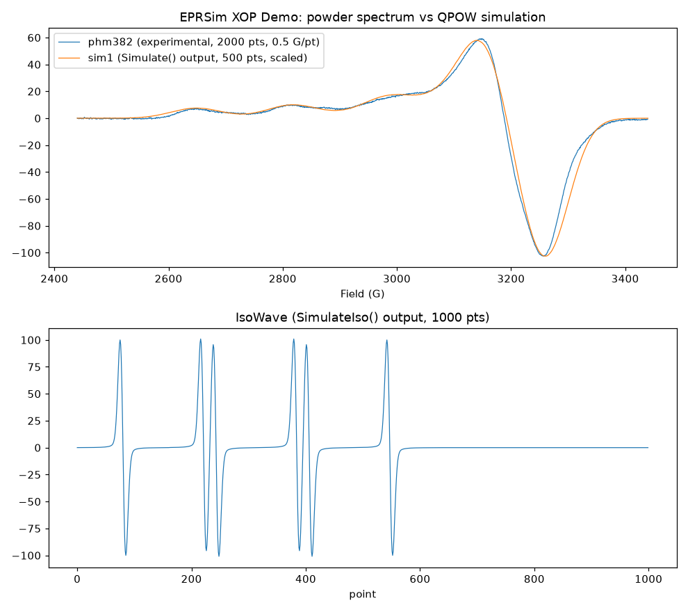
Running it again

The params values above (g = 2.036, 2.036, 2.245; A = 40, 40, 525 MHz; natural-abundance copper; 9.105 GHz; 2440–3440 G) fed to the open-source Python package EPRsim on 6 Sep 2026. Every hyperfine line lands where QPOW put it; the widths agree once the linewidth is expressed in EPRsim's convention (8.0 mT Gaussian FWHM here, against QPOW's 130/130/160 MHz plus its strain terms). Correlation with sim1: 0.995. The script is resim_with_EPRsim.py (raw); it took 0.04 s.

The plug-in itself will not run anywhere current: it is 68K/PowerPC code for Classic Mac OS and Igor Pro 2 or 3. The experiment, however, opens in today's Igor Pro (the macros, tables, notebooks and graphs come back; Simulate() is simply missing, so the graphs show the saved waves). The parameters above map one to one onto QPOW's input, and the same calculation is what EasySpin (MATLAB) and the Python package EPRsim do today.